Machine learning - Regression - Simple Linear Regression
Simple linear regression es una ecuacion de primer grado. Para calcular los mejores coeficientes usa el metodo Ordinary least squares
y=b + cx

- y	variable dependiente
- b	constant y-intercept
- c	slope coeficient
- x	variable independiente
Importing the libraries
import numpy as np 			# trabajo con arrays
import matplotlib.pyplot as plt 	# para hacer gráficos
import pandas as pd 			# importar los datasets, la matriz de características y el vector de variable dependiente
Importing the dataset
dataset = pd.read_csv('Data.csv') 	# cargo el dataset
print(dataset)
    YearsExperience    Salary
0               1.1   39343.0
1               1.3   46205.0
2               1.5   37731.0
3               2.0   43525.0
4               2.2   39891.0
5               2.9   56642.0
6               3.0   60150.0
7               3.2   54445.0
8               3.2   64445.0
9               3.7   57189.0
10              3.9   63218.0
11              4.0   55794.0
12              4.0   56957.0
13              4.1   57081.0
14              4.5   61111.0
15              4.9   67938.0
16              5.1   66029.0
17              5.3   83088.0
18              5.9   81363.0
19              6.0   93940.0
20              6.8   91738.0
21              7.1   98273.0
22              7.9  101302.0
23              8.2  113812.0
24              8.7  109431.0
25              9.0  105582.0
26              9.5  116969.0
27              9.6  112635.0
28             10.3  122391.0
29             10.5  121872.0


X = dataset.iloc[:, :-1].values 	# pongo en el panda dataset X todas las filas de todas las columnas menos la última porque en ella está la variable dependiente
y = dataset.iloc[:, -1].values 		# pongo en el panda dataset y todas las filas de la ultima columna

print(X)
[[ 1.1]
 [ 1.3]
 [ 1.5]
 [ 2. ]
 [ 2.2]
 [ 2.9]
 [ 3. ]
 [ 3.2]
 [ 3.2]
 [ 3.7]
 [ 3.9]
 [ 4. ]
 [ 4. ]
 [ 4.1]
 [ 4.5]
 [ 4.9]
 [ 5.1]
 [ 5.3]
 [ 5.9]
 [ 6. ]
 [ 6.8]
 [ 7.1]
 [ 7.9]
 [ 8.2]
 [ 8.7]
 [ 9. ]
 [ 9.5]
 [ 9.6]
 [10.3]
 [10.5]]

print(y)
[ 39343.  46205.  37731.  43525.  39891.  56642.  60150.  54445.  64445.
  57189.  63218.  55794.  56957.  57081.  61111.  67938.  66029.  83088.
  81363.  93940.  91738.  98273. 101302. 113812. 109431. 105582. 116969.
Splitting the dataset into the Training set and Test set
Se suelen crear 4 datasets
- X_train 66% para entrenar el modelo
- Y_train las respuestas de X_train
- X_test 33% para comprobar el modelo
- Y_test las respuestas del modelo


from sklearn.model_selection import train_test_split
X_train, X_test, y_train, y_test = train_test_split(X, y, test_size = 1/3, random_state = 0)	#0.33 dedico el 33% a test

print(X_train)
[ 2.9]
 [ 5.1]
 [ 3.2]
 [ 4.5]
 [ 8.2]
 [ 6.8]
 [ 1.3]
 [10.5]
 [ 3. ]
 [ 2.2]
 [ 5.9]
 [ 6. ]
 [ 3.7]
 [ 3.2]
 [ 9. ]
 [ 2. ]
 [ 1.1]
 [ 7.1]
 [ 4.9]
 [ 4. ]]

print(X_test)
[[ 1.5]
 [10.3]
 [ 4.1]
 [ 3.9]
 [ 9.5]
 [ 8.7]
 [ 9.6]
 [ 4. ]
 [ 5.3]
 [ 7.9]]

print(y_train)
[ 56642.  66029.  64445.  61111. 113812.  91738.  46205. 121872.  60150.
  39891.  81363.  93940.  57189.  54445. 105582.  43525.  39343.  98273.
  67938.  56957.]

print(y_test)
[ 37731. 122391.  57081.  63218. 116969. 109431. 112635.  55794.  83088.
 101302.]
Training the Simple Linear Regression model on the Training set
from sklearn.linear_model import LinearRegression	# importo la clase LinearRegression de la libreria sklearn del modulo linear_model
regressor = LinearRegression()				# creo un objeto de la clase LinearRegression
regressor.fit(X_train, y_train)				# fit = entreno el modelo con los datasets de train
Predicting the Test set results
y_pred = regressor.predict(X_test) # obtengo los resultados de X_test
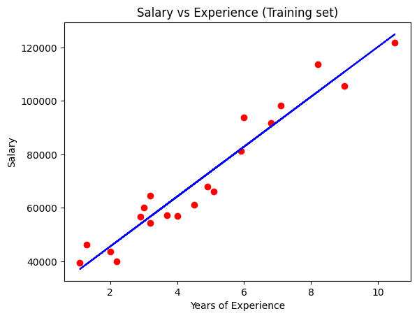
Visualising the Training set results
plt.scatter(X_train, y_train, color = 'red')			# dibujo en puntos rojos los datos de training
plt.plot(X_train, regressor.predict(X_train), color = 'blue')	# dibujo en azul el modelo
plt.title('Salary vs Experience (Training set)')
plt.xlabel('Years of Experience')
plt.ylabel('Salary')
plt.show()
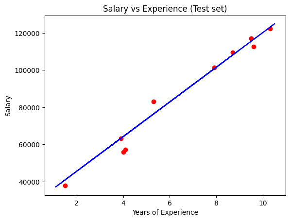
Visualising the Test set results
plt.scatter(X_test, y_test, color = 'red')			# dibujo enrojo los datos de testeo
plt.plot(X_train, regressor.predict(X_train), color = 'blue')	# dibujo en azul el model,uso X_train porque el modelo es el mismo que para X_test
plt.title('Salary vs Experience (Test set)')
plt.xlabel('Years of Experience')
plt.ylabel('Salary')
plt.show()
Making a single prediction (for example the salary of an employee with 12 years of experience)
print(regressor.predict([[12]]))	# los 2 [[ es porque el modelo espera un array de 2 dimensiones
[138967.5015615]
Getting the final linear regression equation with the values of the coefficients
print(regressor.coef_)
print(regressor.intercept_)

[9345.94244312]
26816.192244031183


Así que el modelo queda Salario = egressor.coef_ x YearsOfExperenia + regressor.intercept_
Salario = 9345.94244312 x YearsOfExperenia + 26816.192244031183